Frozen
Here is an active version
Android Accelerometer and Low-pass Filter
A sensors in our mobile phones have, among other things, an imperfect output signal quality. Well, it’s difficult to do something with the hardware, but one can play with software digital signal filters.
A bit of theory
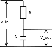
Consider the simplest low-pass filter:

The voltage drop across the resistor and the current through it are connected:
On the other hand, the definition of capacity implies:
where \(Q_c(t)\) - charge of the capacitor at time \(t\). Then \(i(t)=C\frac{V_{out}(t)}{dt}\) and finally the filter is described by the equation:
One can go to a discrete form. Assume that samples of the input and output signals are taken at regular intervals \( \Delta T\), sequence \(\lbrace x_1, x_2, x_3, \ldots x_n\rbrace\) - input signal \(V_{in}\), \(\lbrace y_1, y_2, y_3, \ldots y_n\rbrace\) - output signal \(V_{out}\), then:
or
\(\alpha=\frac{RC}{RC+\Delta T}\) - coefficient of smoothing. From \(RC\), the filter smoothing frequency \(f_c = \frac{1}{2\pi RC}\) is determined, that is, the frequency above which the signal begins to smooth out.
Filter in Maxima
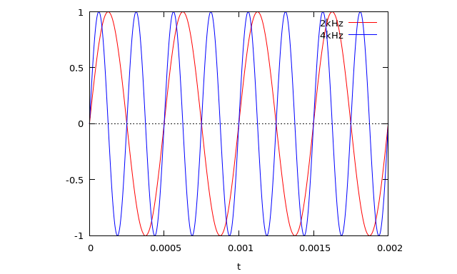
Suppose we have at the input a useful signal with a frequency of 2 kHz and noise with a frequency of 4 kHz:

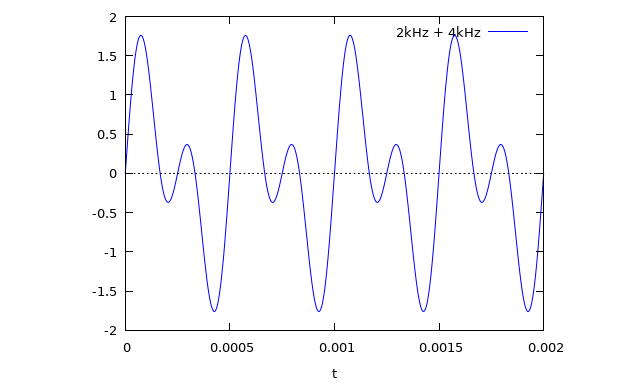
Naturally, the filter input receives a total signal:

Signal and noise are given by functions:
kH2(t):=sin(2*%pi*2000*t)$
kH4(t):=sin(2*%pi*4000*t)$
In Maxima we can describe the input data with two lists of values, tl - time counts of 100 intervals of 0.00005 seconds, kH2lkH4l - a list of input values \(x_i\):
tl:makelist(i / (100 * 500), i, 0, 100)$
kH2lkH4l:makelist(kH4(i / (100 * 500)) + kH2(i / (100 * 500)), i, 0, 100)$
The filter function itself consists of a recursive part that literally repeats \(y_i=\alpha y_{i-1} + (1 - \alpha)x_i\):
lowpass_rec(x, alpha):=
  if length(x) = 1 then
    [(1 - alpha) * first(x)]
  else block([y],
    y: lowpass_rec(rest(x), alpha),
    return(cons(alpha * first(y) + (1 - alpha) * first(x), y)))$
and the entry point:
lowpass(x, alpha):=reverse(lowpass_rec(reverse(x), alpha))$
\(\Delta T=0.00005\) is fixed and is defined by frequency of data receipt from the sensor. The smoothing frequency is 3kHz: \(f_c=\frac{1}{2\pi RC}=3000\)Hz.
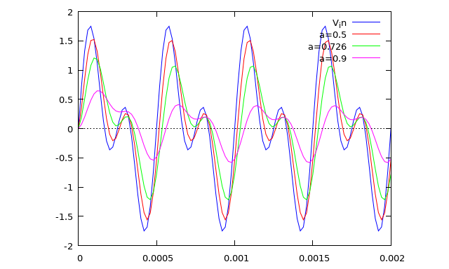
Let’s see how the filter works with this value of \(\alpha\) together with the others.
plot2d([[discrete, tl, kH2lkH4l], [discrete, tl, lowpass(kH2lkH4l, 0.5)],
        [discrete, tl, lowpass(kH2lkH4l, 0.7262210965743948)],
        [discrete, tl, lowpass(kH2lkH4l, 0.9)]],
        [legend, "V_in", "a=0.5", "a=0.726", "a=0.9"])$

For the other values of \(\alpha \), the boundary frequencies of this filter are equal, respectively:
Hz - all passes through the filter practically unchanged.
Hz - the filter actively smoothes both our signal in 2kHz and noise in 4kHz.
Afterword
It seems that one can already insert this filter as there is somewhere like:
  @Override
    public void onSensorChanged(SensorEvent event)
    {
\(\ldots\) and be disappointed. The reason is in \(\Delta T \) or in the sampling period, which varies from model to model, and during the program operation can vary quite significantly. And for a fixed \(\alpha \) this will change the operating frequency of the filter. So \(\alpha \) must be dynamic, we’ll discuss it next time. ![]()

